Chapter 6 Evolutionary Mechanisms II: Mutation, Genetic Drift, Migration, and Non-Random Mating

Simulations in the previous chapter revealed complex evolutionary responses to selection. Contrary to common beliefs, selection does not always drive beneficial alleles to fixation; selection can maintain allele frequencies at intermediate equilibria, or even cause fixation of alleles that confer a fitness cost. While the outcomes of simulations align well with empirical studies of selection, the mathematical models employed in Chapter 5 made some critical assumptions that may not hold up in natural populations: we assumed that there was no mutation, an infinite population size, a single population that is not connected to others, and random mating among all genotypes. All of these assumptions relate to other evolutionary forces that can bias the frequency of particular genotypes and skew allele frequencies across generations. In this chapter, we explore how the different evolutionary forces impact allele frequencies in populations, and how they interact with selection in natural settings.

6.1 Mutation: The Force Creating Novelty

Mutations provide the raw material upon which selection can act (Chapter 4). At any given locus, mutation can cause transitions between alleles (A₁ to A₂, or vice versa), or introduce a new allele (A₃). Despite the critical importance of mutation to evolutionary processes, mutation by itself is a weak evolutionary force. Because mutation rates are low, mutation at any locus only causes minute changes in allele frequency across generations.

Nonetheless, there are important interactions between mutation and selection—especially in terms of the persistence of deleterious alleles in a population. In the absence of mutation, selection keeps a recessive deleterious gene at a very low frequency (black line in Figure 6.1). But as selection removes deleterious alleles in every generation, mutation continuously reintroduces them. When the rate of elimination of deleterious alleles is equal to the rate of mutation, the frequency of an allele is at an equilibrium, called the mutation-selection balance. Assuming a dominant-recessive mode of inheritance (w_AA = w_Aa), the frequency of a deleterious allele at equilibrium is given by the mutation rate (𝜇) and the strength of selection (s):

\[\begin{align} q=\sqrt{𝜇/s} \tag{6.1} \end{align}\]

Consequently, the frequency of a deleterious allele depends on its mutation rate and the strength of selection against it. The equilibrium frequency of a deleterious allele increases with increasing mutation rate or with decreasing strength of selection, as illustrated in Figure 6.1.

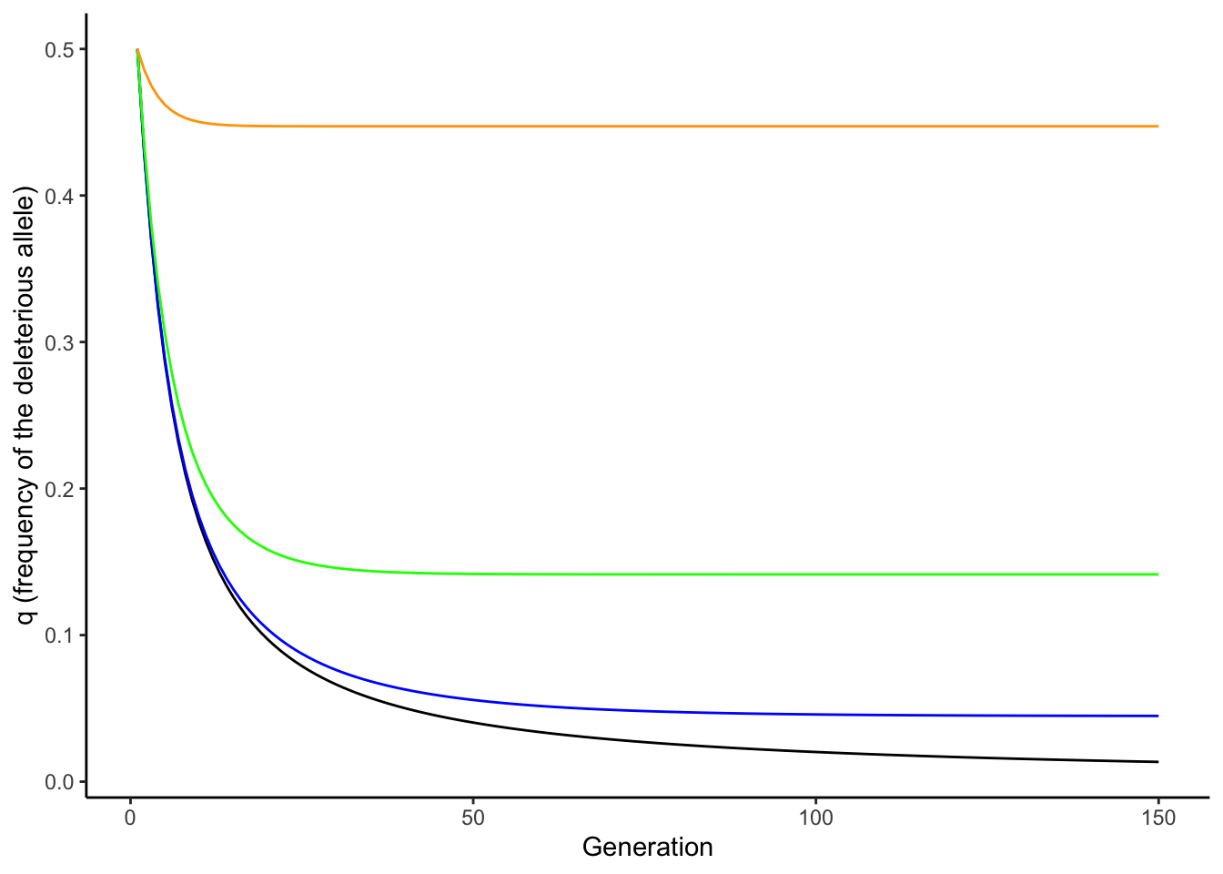
Figure 6.1: In absence of mutation, selection maintains a recessive deleterious allele at low frequency (black line). As mutation rate increases, the equilibrium frequency of the deleterious allele increases (blue: mu=0.001; green: mu=0.01; orange: mu=0.1). The strength of selection was 0.5 for all simulations.

Note that Equation (6.1) can be used to make inferences about mutation rates, when equilibrium allele frequencies and the strength of selection are known (because 𝜇=q²*s). Accordingly, the principle of mutation-selection balance is an important null model that describes the relationship between selection, mutation, and allele frequencies, and it can be applied to study the prevalence of heritable diseases.

6.2 Genetic Drift: The Random Force

Models of selection are completely deterministic because they assume infinite population sizes. No matter how many times you run a simulation with the same parameters, you will always get exactly the same result. In reality, however, population sizes are finite. While many species on the planet do indeed have very large populations (in the order of millions and billions and even trillions), others are comparatively rare. Some rare species have naturally low populations sizes with historically restricted distributions (Figure 6.2); others have declined in recent decades due to anthropogenic environmental change. Species with small or declining population sizes are the focus of conservation biology, which applies evolutionary principles to develop strategies for population management.

Figure 6.2: The Devils Hole pupfish (Cyprinodon diabolis) is one of the rarest vertebrates on the planet. The species is endemic to the tiny Devil’s Hole well, which is located within the Ash Meadows National Wildlife Refuge, Nevada. Since the start of population surveys, the maximum population size recorded was 553, and the lowest population size was just 38 individuals in 2006. Photo by Olin Feuerbacher, CC BY 2.0.

When population sizes are finite—and especially when they are small—random chance affects evolutionary dynamics. These changes in allele frequencies across generations caused by random events are called genetic drift. While selection is differential reproductive success caused by differential performance of variants, genetic drift is differential reproductive success that just happens. In contrast to selection, which tends to increase average fitness across generations, genetic drift does not lead to adaptation. Due to the random nature of genetic drift, populations subject to it evolve on distinct trajectories. So, if you re-run simulations allowing for drift with the same parameters, you will get a unique evolutionary path every single time. The random nature of drift assures that no evolutionary trajectory is like another.

At the most basic level, evolution by genetic drift happens as a consequence of sampling error across generations. If you imagine a locus with two alleles (\(A_1\) and \(A_2\)) of equal frequency, the theoretically predicted allele frequencies under Hardy-Weinberg conditions in the next generation are of course p=q=0.5. However, chance might cause significant deviations from theoretical expectations in reality. Every individual in the population essentially has a 50% chance to inherit the \(A_1\) allele on its first chromosome, and a 50% chance to inherit the \(A_1\) allele on its second chromosome. In other words, the genotype an individual inherits in absence of selection is equivalent to two coin tosses (one for each allele inherited), where the probability for receiving a particular genotype is dependent on the allele frequencies in the population. We can simulate this in R using the rbinom() function, with the allele frequency (p) and the population size (N) as input variables. So for the Devil’s Hole pupfish (Figure 6.2), with its low-bound population size of 38, the simulated allele frequency in the next generation is:

N=38
p=0.5
rbinom(1, size=2*N, prob=p)/(2*N)

## [1] 0.5526316

If we repeat this simulation 1,000 times, you can see that there can be substantial deviations from the predicted allele frequency of p=0.5 (Figure 6.3). Only about 10% of observations fall within the predicted 0.5-bin, and the frequency of A can be as low as 0.3 and as high as 0.7 just because of random chance. That is a massive shift in allele frequency across a single generation.

As you know from experience, the number of coin tosses impacts how close a result matches the theoretical predictions. If you toss your coin ten times, you may get tails eight times, which represents a 60% deviation from the theoretical prediction. However, the more often you toss your coin, the closer your overall frequency of tails will get to the predicted 50%. The same principle applies to the effects of genetic drift as a function of population size. When population sizes are small, genetic drift can induce substantial deviations from theoretical predictions, but the effects of drift get smaller as population size increases. Using the same simulation as above—but with a population size of 1,000—reveals that observed allele frequencies align much better with theoretical predictions, with a spread of observed allele frequencies of \(A_1\) between 0.46 and 0.54 (Figure 6.3).

So how exactly does population size impact the strength of genetic drift? If a new mutation arises in a population of diploid organisms with a population size of N, the frequency of the new allele is 1/2N. Each neutral allele has the same chance of drifting to fixation, which is equal to the allele frequency. Hence, the likelihood that the new allele gets fixed in a population is 1/2N. Correspondingly, novel alleles are more likely to get fixed by chance in small populations.

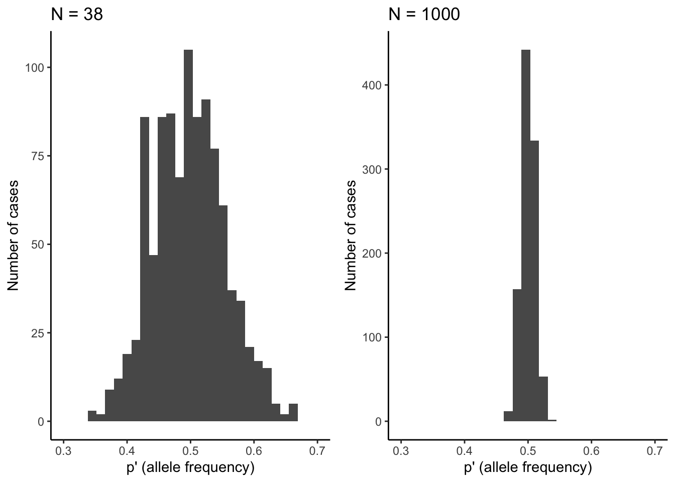
Figure 6.3: Observed distributions of allele frequencies by randomly selecting alleles (\(A_1\) or \(A_2\)) from a pool with equal allele frequencies (p=0.5). The deviation from theoretical expectations are much larger for the small population (N=38) than for the larger population (N=1,000). This illustrates how the strenth of genetic drift declines as a function of population size.

Effective Population Size

The total population size (census population size) in natural populations is not the same as the effective population size (N_e), which is the size of the breeding population. Effective population size takes into consideration that many individuals that reach adulthood never breed in natural populations. Consequently, effective population size is almost always smaller than the census population size. Effective population size is particularly impacted by deviations from 1:1 sex ratios. In such cases, effective population size can be estimated as

\[\begin{align} N_e = \frac{4N_mN_f}{N_m+N_f} \tag{6.2} \end{align}\]

where N_m is the number of males and N_f the number of females. If you assume a census population of 100 with equal sex ratio, N_e is 100. If you assume a sex ratio of 1:9, N_e drops to just 36. Distinguishing between N and N_e is important for conservation biology and many population genetic analyses related to genetic drift and inbreeding. For example, when N_e is significantly smaller than N, the probability of fixation of an allele in response to drift can be much higher than estimated by census population sizes.

Besides sampling error, genetic drift can also have profound impacts on allele frequencies when there are rapid reductions in population size. In general, we distinguish between two scenarios: (1) Population bottlenecks occur when catastrophic events (large-scale wild fires, floods, etc.) drastically reduce the size of a population. In such instances, survival is less dependent on individuals’ traits (that would be selection) than individuals being in the right place at the right time. Hence, the allelic composition of the generation after a bottleneck largely reflects a random subsample of the original population. (2) Founder effects occur when a small subset of a population disperses into a new area and founds a new population. In that case, only a random subset of alleles travels along with the founding individuals. Founder effects are particularly important in island populations, where species expand their range in a step-wise fashion along island chains. This can lead to serial founder effects with continuous loss of genetic diversity (Figure 6.4).

Figure 6.4: Allelic richness in populations of monarch butterflies (Danaus plexippus). The original population from the United States exhibits the highest levels of allelic richness. Allelic richness declined in a step-wise fashion as butterflies first colonized Hawaii and then other islands throughout the Pacific. Data from Pierce et al. (2014).

6.3 Migration: The Homogenizing Force

Our view of evolutionary processes so far has assumed that populations are relatively homogenous, with random mating among all individuals contained within (i.e., panmixia). More often than not, however, species consist of many populations that inhabit suitable habitat patches and are separated by less favorable environmental conditions (Figure 6.5A-B). Such partial isolation can cause differentiation among populations, either because genetic drift impacts allele frequencies differently across populations, or because variation in environmental conditions among populations favors different individuals with different genotypes. But despite some degree of isolation, populations within a species are typically connected through migration. Migration can be unidirectional or bidirectional, and can vary in strength (i.e., the number of migrating individuals relative to the population size). Migration rates are typically higher between proximate (nearby) populations than between populations that are far apart—a phenomenon known as isolation by distance.

Definition: Gene Flow

Population geneticists usually refer to migration as “gene flow.” Gene flow is simply the transfer of genetic material among populations.

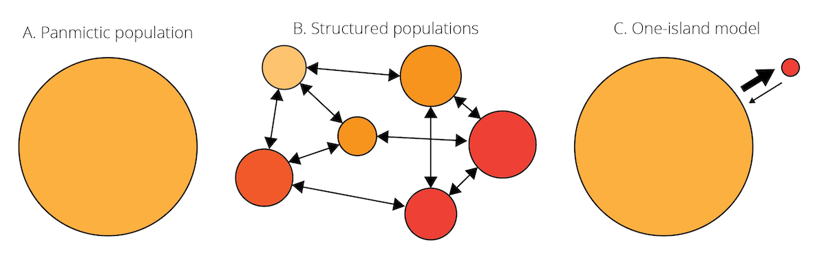
Figure 6.5: A. Species are often assumed to be relatively homogenous units with panmixia. B. However, species can also consist of structured populations that are somewhat differentiated but still connected by migration. Variation in color indicates population differentiation; arrows represent patterns of migration among populations. C. Schematic of the one-island migration model.

Migration is an evolutionary force because it can impact the genetic composition of populations. Migrants may carry novel alleles from one population to another, acting similar to mutation in terms of introducing new genetic variation. Even in the absence of novel alleles, migration between differentiated population causes changes in allele frequencies. In the absence of other evolutionary forces, it homogenizes the genetic composition of populations connected through migration. To illustrate this, let’s consider a simple scenario known as the one-island migration model (Figure 6.5C). The model assumes two populations: a large mainland population and a small island population. Even if the number of individuals migrating in either direction is the same, the input of island individuals arriving in the mainland population is negligible because of its large size. In contrast, because of the small island population, individuals from the mainland arriving on the island can significantly impact allele frequencies, if allele frequencies differ between populations. In this case, island allele frequencies after a migration event (p_i’) can be described as a function of island allele frequencies before a migration event (p_i), mainland allele frequencies (p_m), and the migration rate (m):

\[\begin{align} p_i' = (1-m)p_i+mp_m \tag{6.3} \\ 𝚫p_i=p_i'-p_i=m(p_m-p_i) \tag{6.4} \end{align}\]

Applying Equation (6.3) and calculating island allele frequencies across multiple generations reveals the genetic effect of migration: migration from the mainland to the island changes p_i until it is equal to p_m, and the rate of migration dictates the speed at which this conversion happens. In other words, migration homogenizes the allele frequencies across populations.

6.3.1 Interactions Between Migration and Selection

Similar to mutation, migration can introduce new genetic variants into a population upon which selection can act. Hence, human-facilitated migration is sometimes used as a tool in conservation biology, where new individuals are introduced into populations of endangered species suffering from low genetic diversity and inbreeding. This practice is also known as genetic rescue. In many instances, however, migration actually counteracts the effects of selection. Imagine two adjacent populations that are exposed to different environmental conditions. In every generation, selection favors alleles that mediate adaptation to the local conditions. But if there is migration between the two populations, new maladaptive alleles are continuously introduced from the other population. Hence, migration can prevent local adaptation of populations. Adaptive divergence between populations is only possible if the effect of divergent selection is stronger than the homogenizing force of migration (Figure 6.6).

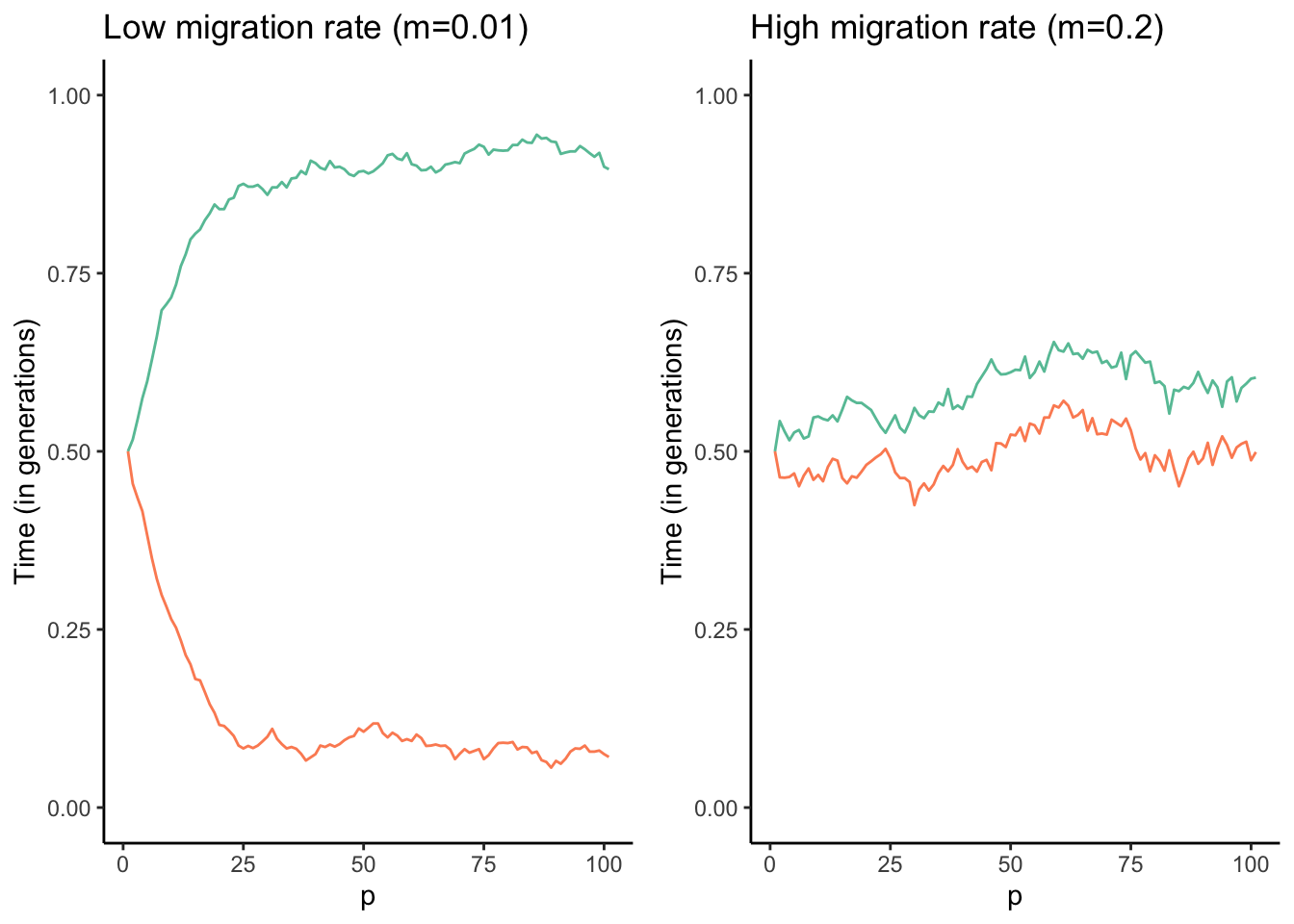
Figure 6.6: Results of a combined simulation of drift, selection, and migration. The optimal allele frequency for population 1 (red) is p=1, and the optimal frequency for population 2 (blue) is p=0. The two models ran were identical except for the migration rate between the two populations. As you can see, populations approach their respective optimal allele frequencies when migration rates are low (left graph). In contrast, higher migration rates continuously homogenize allele frequencies across the populations, and accordingly allele frequencies hover around p=0.5 (right graph).

Evidence for the tension between selection and migration is also observed in natural populations. Remember the stick insects of the genus Timema that we got to know in Chapter 2? As you might recall, different populations of T. cristinae are adapting to different host plants—either broad-leafed species of the genus Ceanothus or needle-leafed species of the genus Adenostoma. Populations adapted to Ceanothus are uniformly colored for optimal camouflage; those adapted to Adenostoma exhibit a dorsal stripe to mimic the needle-like leaves (see Figure 2.4). If selection was the only evolutionary force, we would expect the optimal phenotype to eventually become fixed in each population. However, both color forms tend to be present in many T. cristinae populations, and the maladaptive morph can even be more common than the adaptive one. Bolnick and Nosil (2007) were able to show that the high frequency of maladaptive morphs is likely a consequence of migration. If neighboring populations adapted to the opposite host are relatively small, with few migrants arriving in a population, selection is able to keep maladaptive morphs at a low frequency (Figure 6.7). However, when neighboring populations are large and provide a source of many migrating individuals, the frequency of maladaptive morphs can be very high due to continuous reintroduction (Figure 6.7).

Figure 6.7: The frequency of maladaptive morphs in Timema stick insects adapted to different plant hosts (Ceanothus and Adenostoma) is directly related to the size of neighboring populations that are a source of migrating individuals. Data from Bolnick & Nosil (2007).

6.4 Non-Random Mating: Not Much of a Force

The last evolutionary force that we need to discuss is non-random mating. Non-random mating occurs when the probability that two individuals in a population will mate is not the same for all possible combinations of genotypes. Non-random mating can be assortative, when individuals are more likely to mate with similar individuals (e.g., individuals having the same genotype or phenotype), or it can be disassortative, when individuals prefer to mate with dissimilar individuals. Technically speaking, non-random mating is not an evolutionary force, because—unlike mutation, selection, drift, and migration—it does not actually cause any change in allele frequencies across generations. It does, however, cause deviations from Hardy-Weinberg assumptions, because the frequency of genotypes do not match Hardy-Weinberg predictions when non-random mating is present. Therefore, non-random mating can have some indirect consequences for evolution.

One of the most common forms of non-random mating is inbreeding, where offspring are produced by individuals that are closely related. The epitome of inbreeding is selfing (self-fertilization), which essentially represents strict genotype-specific assortative mating and is particularly common in plants. If we assume a single, biallelic locus A, possible matings during selfing include AA x AA, Aa x Aa, and aa x aa. The consequences of selfing on the genotype frequencies across generations are depicted in Figure 6.8. As you can see, the frequency of heterozygotes declines rapidly until they are virtually gone after just 10 generations. This is because neither the self-crosses of AA and aa yield any heterozygotes, and self-crosses of Aa yield 50% homozygotes. Accordingly, the frequency of heterozygotes is halved in every generation.

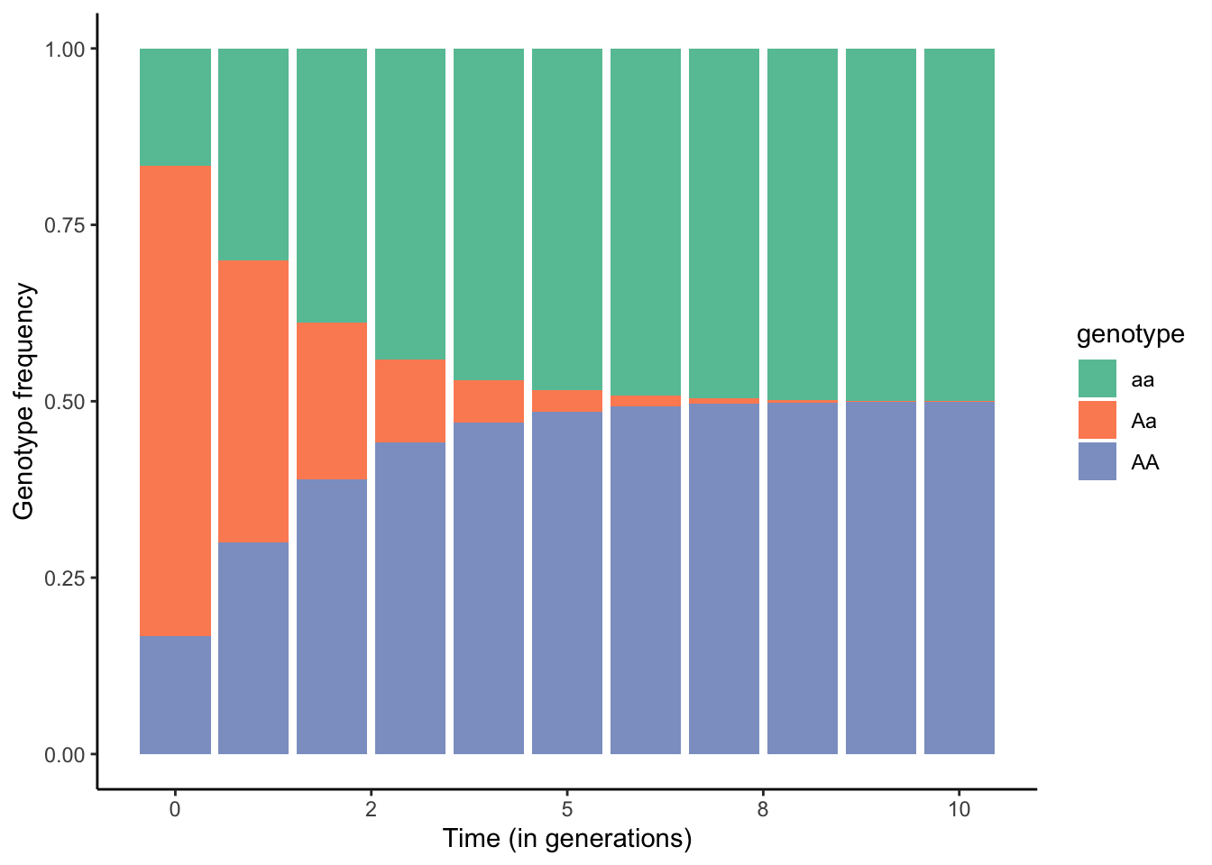
Figure 6.8: Changes in genotype frequencies across generations when all individuals in a population self-fertilize.

The degree of inbreeding can be described by the coefficient of inbreeding (F), which calculates the probability that two copies of an allele have been inherited from an ancestor common to both the mother and the father. You can find some examples for inbreeding coefficients in Table 6.1. Once we know F for a population, we can account for the effects of inbreeding on genotype frequencies by modifying the original Hardy-Weinberg formulas:

\[\begin{align} fr({A_1A_1}) = p^2(1-F)+pF \tag{6.5} \\ fr({A_1A_2}) = 2pq(1-F) \tag{6.6} \\ fr({A_2A_2}) = q^2(1-F)+qF \tag{6.7} \end{align}\]

Similarly, we can calculate the heterozygosity after inbreeding (H’) based on F and the heterozygosity under Hardy-Weinberg assumptions (H₀):

\[\begin{align} H' = H_0(1-F) \tag{6.8} \end{align}\]

Expected and Observed Heterozygosity

Heterozygosity is a measure of genetic variability in a population. While there are multiple metrics of heterozygosity, the most commonly used one is expected heterozygosity H_E (also known as gene diversity, D). For a single locus with k alleles, expected heterozygosity is defined as:

\[\begin{align} H_E = 1-\sum_{i=1}^k p_i^2 \tag{6.9} \end{align}\]

Hence, for a bi-allelic locus with allele frequencies p and q, expected heterozygosity is:

\[\begin{align} H_E = 1-(p^2 + q^2) \tag{6.10} \end{align}\]

H_E can range from zero (when a population is fixed for a single allele) to almost 1 (when a locus has a large number of alleles with the same frequency). In practice, we can apply expected heterozygosity as a null model for inbreeding. Based on population level genotype data, we can calculate observed heterozygosity (H_O) and allele frequencies, which allow us to also calculate expected heterozygosity (H_E). If H_E=H_O, the observed heterozygosity matches the theoretical predictions, meaning that all Hardy-Weinberg assumptions are met. If H_E≠H_O, some evolutionary force must be acting on the particular locus. Most commonly, H_E>>H_O can be an indicator of inbreeding in a population.

The degree of inbreeding is often quantified based on many loci in the genome, not just one. For m loci, genome-wide heterozygosity (F) is:

\[\begin{align} F = 1-\frac{1}{m} \sum_{l=1}^m \sum_{i=1}^k p_i^2 \tag{6.11} \end{align}\]

Equation (6.8) allows us to simulate the effects of different levels of inbreeding on the observed heterozygosity across successive generations. As you can see in Figure 6.9, the rate of decline in heterozygosity across generations is dependent on F, and declines can be rapid when inbreeding is common. Declines in heterozygosity are particularly common in small populations where the pool of potential partners is limited, inadvertently leading to mating between related individuals. This is also the case for many managed populations, including those associated with captive breeding programs for endangered species. Hence, many species maintenance programs strategically share individuals for breeding across institutions to avoid inbreeding.

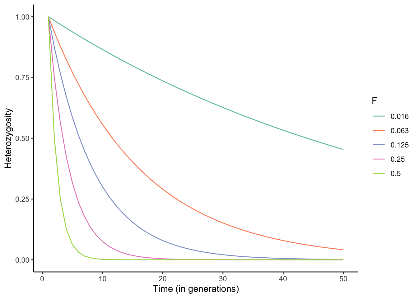
Figure 6.9: Rates of decline in heterozygosity for different levels of inbreeding described by F (also see Table 6.1).

6.5 References

• Bolnick DI, P Nosil (2007). Natural selection in populations subject to a migration load. Evolution 61, 2229–2243.

• Charlesworth B (2009). Fundamental concepts in genetics: effective population size and patterns of molecular evolution and variation. Nature Reviews Genetics 10, 195–205.

• Dyer RJ (2017). Applied Population Genetics.

• Pemberton JM, PE Ellis, JG Pilkington, C Bérénos (2017). Inbreeding depression by environment interactions in a free-living mammal population. Heredity 118, 64–77.

• Pierce AA, MP Zalucki,M Bangura, M Udawatta, MR Kronforst, S Altizer … JC de Roode (2014). Serial founder effects and genetic differentiation during worldwide range expansion of monarch butterflies. Proceedings of the Royal Society B 281, 20142230.